First of all EigenValues and EigenVectors are part of Linear Algebra. The branch of Mathematics which deals with linear equations, matrices, and vectors. The prime focus of the branch is vector spaces and linear mappings between vector spaces. The more discrete way will be saying that Linear Algebra provides various ways of solving and manipulating the world of linear equations.

Do you want to learn python from scratch? Then Intellipaat python course helps you to master python from basics to advance level taught by industry experts.

Let’s have a brief of each complex term for the starters of this article.

So, what are Linear Equations, Matrices, and Vectors? Spend some time, till then let me tell you another intriguing thing.

Python is the next intriguing thing. It’s so awesome that it can take care of every job and task of you, in the most efficient way. It has firmed its feet in every domain of the Information Technology field. From small scale IT industry to the big tycoons of the industry, Python has marked its territory, and it’s not halting, extending its boundaries beyond the horizon. The Python Certification will unleash all of its complexities by lifting the veil of ignorance and turn it into your dexterities.

Now back to our query; let’s approach them one by one:-

1. Linear Equations – The combination or mixture of two unknowns with mathematical operators to operate on, and finally equated to 0 to know the results; basically, the approach of a linear polynomial is followed.
   Example:

   X + Y + c = 0

   X and Y are the two unknowns and c is the constant equated to 0.

2. Matrices – the matrix is an array of numbers. Array – a collection of homogeneous values. The pictorial representation in a table form. Why do we then need Matrices? Because the data is represented in the most compact form and you can automate the operations on it, and even one can manipulate it to his best use.
3. Vectors – Since from high school the definition of vectors is that quantity which has magnitude and direction. You can move forward or backward given the direction of the quantity.

Now let’s see the concept of EigenValues and EigenVectors:

EigenValues and EigenVectors are extensively used in transformation purposes like skewing, enlarging, shrinking, shearing, etc. of the figures or shapes or images. How to attain the stability in Mechanical Engineering and architecture is another application of both of these!

Remember whensoever they (EigenValues and EigenVectors) will come, they’ll be seen all together. None of them can live without the one-another, as the basic equation laying down the definition of both will clarify this Collusion.

Where A is the matrix, v is an EigenVector, λ (Lambda) is an EigenValue and v is EigenVector.

Moreover, EigenValues/Vectors are the fundamental quantities to study electrical circuits, mechanical systems; in fact, it’s used in Google’s PageRank algorithm. Check this StackExchange link to see some more applications.

Nowadays their application has grown to the field of Artificial Intelligence too. They are extensively used in Deep Learning and in Machine Learning algorithms too, to make the world a better place — strictly in Computer Vision, sound analysis (the detection and recognition) domains.

You might have seen or been familiarized with their application known as Face Recognition or technically EigenFaces or Principal Component Analysis (PCA), and even the error-ellipses. On top of all of this, the Eigendecomposition is the fundamental foundation of the geometric interpretation of covariance matrices.

An EigenVector is a special kind of vector whose direction does not change on linear transformation, doesn’t matter which linear transformation it is.

An EigenValue is the scalar quantity which defines the EigenVector.

Let’s see if the visualizations can help us to understand the terms in a more precise form.

The red lines with black arrows are EigenVectors and are not altering their direction. Here Scaling is applied. The other vectors like the one in yellow color do change.

Suppose we have a vector v (represented as a point) and A is a matrix accompanied by a1 and a2 as columns (depicted as arrows). Now if we have a product of A and v, the resultant is Av a new vector.

python3-matrix

I urge you to visit the site setosa.io to have the visual explanation of the working of the above diagram’s illustration.

The moment you’ll click on the any of the a1 or a2 arrows the redpoint Av changes along with the values in A matrix as well as the resultant Av.

Now let’s built some Python script to make machines understand the concept. By the way, the code is the courtesy of Bhavesh Bhatt.

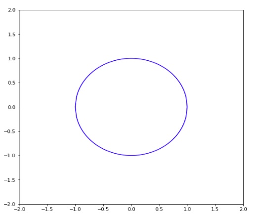
1
2
3
4
5
6
7
8
9
10
11
12
13
14

import numpy as np
import pandas as pd
import matplotlib.pyplot as plt
from pylab import rcParams
%matplotlib inline
rcParams['figure.figsize'] = 8,8
x = np.linspace(-1,1,100)
y1 = np.sqrt(1 - np.square(x))
y2 = -1 * y1
plt.plot(x,y1, 'b')
plt.plot(x,y2, 'b')
plt.xlim([-2, 2])
plt.ylim([-2, 2])
plt.show()

import numpy as np
import pandas as pd
import matplotlib.pyplot as plt
from pylab import rcParams
%matplotlib inline
rcParams['figure.figsize'] = 8,8
x = np.linspace(-1,1,100)
y1 = np.sqrt(1 - np.square(x))
y2 = -1 * y1
plt.plot(x,y1, 'b')
plt.plot(x,y2, 'b')
plt.xlim([-2, 2])
plt.ylim([-2, 2])
plt.show()

python3-circle

1
2
3
4
5
6
7

def transformation(x,y):
    return 9*x + 4*y, 4*x + 3*y
 
x_new1, y_new1 = transformation(x,y1)
x_new2, y_new2 = transformation(x,y2)
plt.plot(x_new1,y_new1, 'r')
plt.plot(x_new2,y_new2, 'r')

def transformation(x,y):
    return 9*x + 4*y, 4*x + 3*y

x_new1, y_new1 = transformation(x,y1)
x_new2, y_new2 = transformation(x,y2)
plt.plot(x_new1,y_new1, 'r')
plt.plot(x_new2,y_new2, 'r')

python3-eclipse

1
2
3
4
5
6
7
8
9
10
11
12
13
14
15
16
17
18
19
20
21
22
23
24
25
26
27
28
29

eig_vals, eig_vecs = np.linalg.eig(np.array([[9,4],[4,3]]))
print('Eigenvectors \n%s' %eig_vecs)
print('\nEigenvalues \n%s' %eig_vals)
=====================================
Eigenvectors 
[[ 0.89442719 -0.4472136 ]
 [ 0.4472136   0.89442719]]
 
Eigenvalues 
[11.  1.]
=====================================
soa = np.array([[0, 0, 
                 eig_vals[0] * eig_vecs[0][0], 
                 eig_vals[0] * eig_vecs[1][0]]])
 
soa1 = np.array([[0, 0, 
                  eig_vals[1] * eig_vecs[0][1], 
                  eig_vals[1] * eig_vecs[1][1]]])
 
X, Y, U, V = zip(*soa)
X1, Y1, U1, V1 = zip(*soa1)
 
plt.plot(x,y1, 'b')
plt.plot(x,y2, 'b')
plt.quiver(X, Y, U, V, angles='xy', scale_units='xy', scale=1)
plt.quiver(X1, Y1, U1, V1, angles='xy', scale_units='xy', scale=1)
plt.xlim([-1, 10])
plt.ylim([-1, 10])
plt.show()

eig_vals, eig_vecs = np.linalg.eig(np.array([[9,4],[4,3]]))
print('Eigenvectors \n%s' %eig_vecs)
print('\nEigenvalues \n%s' %eig_vals)
=====================================
Eigenvectors 
[[ 0.89442719 -0.4472136 ]
 [ 0.4472136   0.89442719]]

Eigenvalues 
[11.  1.]
=====================================
soa = np.array([[0, 0, 
                 eig_vals[0] * eig_vecs[0][0], 
                 eig_vals[0] * eig_vecs[1][0]]])

soa1 = np.array([[0, 0, 
                  eig_vals[1] * eig_vecs[0][1], 
                  eig_vals[1] * eig_vecs[1][1]]])

X, Y, U, V = zip(*soa)
X1, Y1, U1, V1 = zip(*soa1)

plt.plot(x,y1, 'b')
plt.plot(x,y2, 'b')
plt.quiver(X, Y, U, V, angles='xy', scale_units='xy', scale=1)
plt.quiver(X1, Y1, U1, V1, angles='xy', scale_units='xy', scale=1)
plt.xlim([-1, 10])
plt.ylim([-1, 10])
plt.show()

python3-circle-arrow

1
2
3
4
5
6
7
8
9
10
11
12
13
14
15
16

soa = np.array([[0, 0, 
                 eig_vals[0] * eig_vecs[0][0], 
                 eig_vals[0] * eig_vecs[1][0]]])
 
soa1 = np.array([[0, 0, 
                  eig_vals[1] * eig_vecs[0][1], 
                  eig_vals[1] * eig_vecs[1][1]]])
 
X, Y, U, V = zip(*soa)
X1, Y1, U1, V1 = zip(*soa1)
plt.plot(x_new1,y_new1, 'r')
plt.plot(x_new2,y_new2, 'r')
plt.quiver(X, Y, U, V, angles='xy', scale_units='xy', scale=1)
plt.quiver(X1, Y1, U1, V1, angles='xy', scale_units='xy', scale=1)
plt.draw()
plt.show()

soa = np.array([[0, 0, 
                 eig_vals[0] * eig_vecs[0][0], 
                 eig_vals[0] * eig_vecs[1][0]]])

soa1 = np.array([[0, 0, 
                  eig_vals[1] * eig_vecs[0][1], 
                  eig_vals[1] * eig_vecs[1][1]]])

X, Y, U, V = zip(*soa)
X1, Y1, U1, V1 = zip(*soa1)
plt.plot(x_new1,y_new1, 'r')
plt.plot(x_new2,y_new2, 'r')
plt.quiver(X, Y, U, V, angles='xy', scale_units='xy', scale=1)
plt.quiver(X1, Y1, U1, V1, angles='xy', scale_units='xy', scale=1)
plt.draw()
plt.show()

python3-graphs

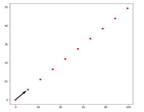
1
2
3
4
5
6
7
8
9
10
11
12
13
14
15
16
17
18
19

x = np.arange(0,10)
print ("Eigen Vectors for Eigen values {} = {} and {}".format(eig_vals[0], 
                                                             eig_vecs[0][0], 
                                                             eig_vecs[1][0]))
==================================================================
Eigen Vectors for Eigen values 11.0 = 0.8944271909999159 and 0.4472135954999579
==================================================================
y = (eig_vecs[1][0] * x )/ eig_vecs[0][0]
 
xnew, ynew = transformation(x,y)
soa = np.array([[0, 0, 
                 eig_vals[0] * eig_vecs[0][0], 
                 eig_vals[0] * eig_vecs[1][0]]])
X, Y, U, V = zip(*soa)
 
plt.quiver(X, Y, U, V, angles='xy', scale_units='xy', scale=1)
plt.scatter(xnew, ynew, color=['red'])
plt.draw()
plt.show()

x = np.arange(0,10)
print ("Eigen Vectors for Eigen values {} = {} and {}".format(eig_vals[0], 
                                                             eig_vecs[0][0], 
                                                             eig_vecs[1][0]))
==================================================================
Eigen Vectors for Eigen values 11.0 = 0.8944271909999159 and 0.4472135954999579
==================================================================
y = (eig_vecs[1][0] * x )/ eig_vecs[0][0]

xnew, ynew = transformation(x,y)
soa = np.array([[0, 0, 
                 eig_vals[0] * eig_vecs[0][0], 
                 eig_vals[0] * eig_vecs[1][0]]])
X, Y, U, V = zip(*soa)

plt.quiver(X, Y, U, V, angles='xy', scale_units='xy', scale=1)
plt.scatter(xnew, ynew, color=['red'])
plt.draw()
plt.show()

python3-draw-a-dash-line

1
2
3
4
5
6
7
8
9
10

xnew, ynew = transformation(x,2*x)
soa = np.array([[0, 0, 
                 10* eig_vals[0] * eig_vecs[0][0], 
                 10 * eig_vals[0] * eig_vecs[1][0]]])
X, Y, U, V = zip(*soa)
 
plt.quiver(X, Y, U, V, angles='xy', scale_units='xy', scale=1)
plt.scatter(xnew, ynew, color=['red'])
plt.draw()
plt.show()

xnew, ynew = transformation(x,2*x)
soa = np.array([[0, 0, 
                 10* eig_vals[0] * eig_vecs[0][0], 
                 10 * eig_vals[0] * eig_vecs[1][0]]])
X, Y, U, V = zip(*soa)

plt.quiver(X, Y, U, V, angles='xy', scale_units='xy', scale=1)
plt.scatter(xnew, ynew, color=['red'])
plt.draw()
plt.show()

python3-dots-line

The Verdict

Python is way more than that one may think of. Today’s professionals just have the gist of the language while the computer scientists know the efficiency of the Python. Moreover, it’s used in every field now and then.

–EOF (The Ultimate Computing & Technology Blog) —